CSCI C343 Data Structures Spring 2024

Lecture: Depth-first Search

Depth-first search chooses to go deeper at each step, following an out-edge from the current vertex to a never-before-seen vertex. If there are no out-edges to never-before-seen vertices, then the search backtracks to the last visited vertex with out-edges to never-before-seen vertices and continues from there.

Show DFS on the following graph, starting at g:

Similar to BFS, DFS traverses a tree, a depth-first tree:

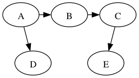
Sometimes all the nodes in a graph are not reachable from the starting node. Consider the following graph, starting at vertex A.

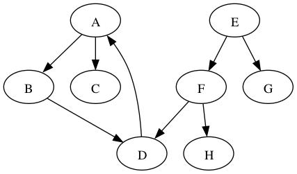
The search from A will reach B, C, and D, but not E, F, G and H. In such situations, one can restart the depth-first search at another vertex. For example, we could restart at the first vertex (alphabetically) that has not yet been visited, which would be E. The depth-first search from E would then reach the remaining vertices, including F, G, and H. But what happens with vertex D? It is reachable from both A and E. The usual thing is to not revisit any nodes, even after restarting. So vertex D would be visited in the search that started from A but not in the search that started from E.

There are two ways to implement DFS. The first is like the algorithm for BFS, but replaces the queue with a stack.

stack.push(start)
while not stack.empty()
  u = stack.pop()
  if not visited[u]
	visited[u] = true
	for v in G.adjacent(u)
	  if not visited[v]
		parent_map[v] = u
		stack.push(v)

The second algorithm for DFS is recursive:

DFS(u, G, parent_map, visited) =
  if not visited[u]
	visited[u] = true
	for v in G.adjacent(u)
	  if not visited[v]
		parent_map[v] = u
		DFS(v, G, parent_map, visited)

DFS and BFS both are good choices for generic search problems, that is, when you’re searching for a vertex.

• BFS may require more storage if the graph has many high degree vertices because the queue gets big.
• On the other hand, if the graph contains long paths, then DFS will use a lot of storage for it’s stack.
• If there are infinitely long paths in the graph, then DFS may not be a good choice.

Student group work

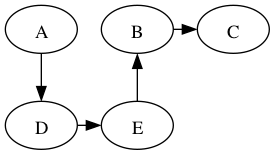
Perform DFS on the following graph

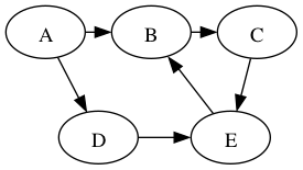
Are any of the DFS trees the same as a BFS tree for this graph? Why not?

(Solution at the bottom of the lecture.)

Edge Categories

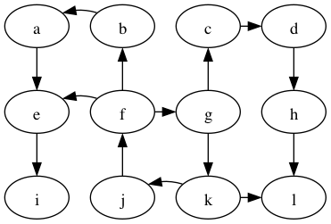
In the following we’ll continue to use this example graph:

We can categorize the edges of the graph with respect to the depth-first tree in the following way:

• tree edge: an edge on the tree, e.g., g → c in the graph above.
• back edge: an edge that connects a descendant to an ancestor with respect to the tree, e.g., f → g.
• forward edge: an edge that connects an ancestor to a descendant wrt. the tree, e.g., f → e
• cross edge: all other edges, e.g., k → l.

A graph has a cycle if and only if there is a back edge.

The DFS algorithm can compute the categories if we use a color scheme to mark the vertices instead of just using a done flag. The colors are:

• white: the vertex has not been discovered
• gray: the vertex has been discovered but some of its descendents have not yet been discovered
• black: the vertex and all of its descendents have been discovered

During DFS, when considering an out-edge of the current vertex, the edge can be categorized as follows:

• the target vertex is white: this is a tree edge
• the target vertex is gray: this is a back edge
• the target vertex is black: this could either be a forward or cross edge

Do the DFS example again but with the white/gray/black colors.

Discover and Finish Times

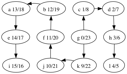
We can discover yet more structure of the graph if we record timestamps on a vertex when it is discovered (turned from white to gray) and when it is finished (turned from gray to black).

This is useful when constructing other algorithms that use DFS, such as topological sort. Here are the discover/finish times for the DFS tree we computed above, shown again below.

What’s the relationship between topological ordering and depth-first search?

Let’s look at the depth-first forest and discover/finish times of the makefile graph.

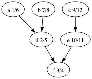
Here’s the vertices ordered by finish time: f,d,a,b,e,c.

That’s the reverse of one of the topological orders: c,e,b,a,d,f.

Why is that? A vertex is finished after every vertex that depends on it is finished. That’s the same as topological ordering except we’ve swapped before for after.

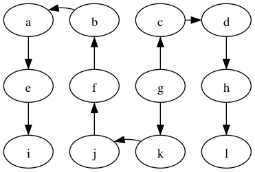
Exercise Solutions

There are multiple depth-first trees: