course-web-page-fall-2022
Course web page for Data Structures H343 Fall 2022
View the Project on GitHub IUDataStructuresCourse/course-web-page-fall-2022
Depth-First Search continued
From last time, example DFS:
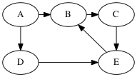
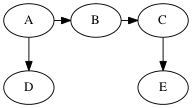
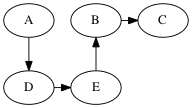
Solutions (there are multiple depth-first trees)
There are two ways to implement DFS. The first is like the algorithm for BFS, but replaces the queue with a stack.
while not stack.empty()
  u = stack.pop()
  for v in G.adjacent(u)
    if not visited[v]
	  visited[v] = true
	  parent[v] = u
	  stack.push(v)
The second algorithm for DFS is recursive:
DFS(u, G, parent, visited) =
  for v in G.adjacent(u)
    if not visited[v]
      visited[v] = true
	  parent[v] = u
	  DFS(v, G, parent, visited)
Edge Categories
In the following we’ll use this example graph:
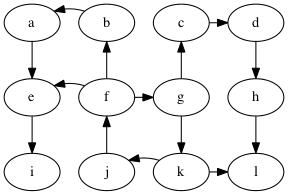
We can categorizes the edges of the graph with respect to the depth-first tree in the following way:
- tree edge: an edge on the tree, e.g., g → c in the graph above.
- back edge: an edge that connects a descendent to an ancestor with respect to the tree, e.g., f → g.
- forward edge: an edge that connects an ancestor to a descendent wrt. the tree, e.g., f → e
- cross edge: all other edges, e.g., k → l.
A graph has a cycle if and only if there is a back edge.
The DFS algorithm can compute the categories if we use a color
scheme to mark the vertices instead of just using a done flag.
The colors are:
- white: the vertex has not been discovered
- gray: the vertex has been discovered but some of its descendents have not yet been discovered
- black: the vertex and all of its descendents have been discovered
During DFS, when considering an out-edge of the current vertex, the edge can be categorized as follows:
- the target vertex is white: this is a tree edge
- the target vertex is gray: this is a back edge
- the target vertex is black: this could either be a forward or cross edge
Do the DFS example again but with the white/gray/black colors.
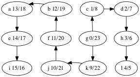
Discover and Finish Times
We can discover yet more structure of the graph if we record timestamps on a vertex when it is discovered (turned from white to gray) and when it is finished (turned from gray to black).
This is useful when constructing other algorithms that use DFS, such as topological sort. Here are the discover/finish times for the DFS tree we computed above, shown again below.
What’s the relationship between topological ordering and depth-first search?
Let’s look at the depth-first forest and discover/finish times of the makefile graph.
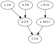
Here’s the vertices ordered by finish time: f,d,a,b,e,c.
That’s the reverse of one of the topological orders: c,e,b,a,d,f.
Why is that? A vertex is finished after every vertex that depends on it is finished. That’s the same as topological ordering except we’ve swapped before for after.
Lecture: Shortest Paths
We have seen the shortest path problem where each edge counts as distance 1 and we used BFS to solve it. Now we consider graphs where each edge has a real number for its weight.
Notation: We write w(u,v) or w(e) for the weight of an edge.
Definition The weight of a path is the sum of the weights of its edges. We also use the term distance for the weight of a path.
So for path p = e₁, e₂, …, eᵣ
w(p) = Σ{i∈1..r} w(eᵢ)
Motivation for the shortest path problem:
- internet packet routing
- driving routes
- minimizing flight duration
As with BFS, we’ll focus on the single-source shortest-paths problem: finding the shortest path from a source vertex to every other vertex in the graph. Other alternatives are:
- Single-destination shortest-paths
- Single-pair shortest-path
- All-pairs shortest-paths
Algorithm Preview
- Bellman-Ford: O(nm)
- Disjktra:
- using min-heap: O((n+m) log(n))
- using Fibonnaci heap: O(n log(n) + m)
- DAG Shortest: O(n+m) (uses topological sort)
Brute force: compute the length of every path
But this is exponential time: there are O(2^n) paths. Here’s a worst-case scenario.
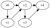
Shortest paths exhibit optimal substructure
That is, a subpath of a shortest path is a shortest path.
More precisely, if you have a shortest path
v₀ →ᵣ vᵢ →p vⱼ →q vk
then the subpath p
vᵢ →p vⱼ
is a shortest path from vᵢ to vⱼ.
Proof. Suppose vᵢ →p vⱼ is not a shortest path from vᵢ to vⱼ. Then we splice the shortest path p’ from vᵢ to vⱼ into the path v₀ → vk to get
v₀ →ᵣ vᵢ →p' vⱼ →q vk
which is a shorter path from v₀ to vk. But that contradicts the assumption that
v₀ →ᵣ vᵢ →p vⱼ →q vk
was a shortest path.
Take away: we can build shortest paths by growing them from smaller shortest paths.
Notation: d(u,v) is the weight of the shortest path from u to v.
Negative-weight edges
Motivation: weak, not very common
Some shortest-path algorithms handle this (Bellman-ford), some do not (Dijkstra, DAG Shortest Paths).
None of them handle graphs with negative-weight cycles, as the notion of shortest-path doesn’t make sense on such graphs.
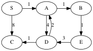
Example:
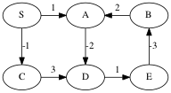
The shortest path from S to C is -1.
The shortest path from S to A is undefined because you can keep going around the cycle A → D → E → B, which has weight -2.
We can avoid negative weights in some situations by shifting weights up.
Triangle Inequality
For all edges u → v, d(s,v) ≤ d(s,u) + w(u,v).
Proof: s → u → v is a path from s to v, and d(s,v) is the weight of the shortest path.
Relaxation
We maintain a current best path length, an upper bound, on the distance to a vertex.
We relax an edge by updating the distance of the target vertex if this edge provides a shorter path to it.
static void relax(Edge e, double[] distance, int[] parent,
                  Map<Edge,Double> weight) {
    if (distance[e.target] > distance[e.source] + weight.get(e)) {
	    distance[e.target] = distance[e.source] + weight.get(e);
		parent[e.target] = e.source;
	}
}
Dijkstra Shortest Paths
Like BFS, the idea is to expand the wavefront of shortest-paths so far.
The challenge is to figure out how to explore paths in the order of their weight. Consider the following graph with the source vertex S.
Growing the shortest paths tree in order of path weight:
        W=0   S

        W=1   S-->A


        W=2   S-->A-->B


        W=3   S-->A-->B
                      |
                      V
                      E

        W=5   S-->A-->B
                  |   |
                  V   V
                  D   E

        W=6   S-->A-->B
                  |   |
                  V   V
              C<--D   E
Dijkstra’s solution is to store all the potential next vertices (those that are adjacent to the tree) in a priority queue ordered by their distance as computed by the current tree plus the weight of the lightest edge to that vertex. Then the minimum of the priority queue gives the next shortest path.
               SPT                  Priority Queue
        W=0    S                    A:1, C:8

        W=1    S---A                B:2, D:5, C:8

        W=2    S---A---B            E:3, D:5, C:8

        W=3    S---A---B            D:5, C:8
                       |
                       |
                       E

        W=5    S---A---B            C:6  (decrease key!)
                   |   |
                   |   |
                   D   E

        W=6    S---A---B
                   |   |
                   |   |
               C---D   E
Student group work: use Dijkstra’s to compute the distances from S to all the other vertices in the following graph.
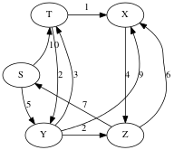
    Answers:

           S: 0
           T: 8
           X: 9
           Y: 5
           Z: 7
Time Complexity of Dijkstra’s Algorithm
- n pushes to the queue: O(n log(n))
- n pops from the queue: O(n log(n))
- m
decrease_keyon the queue: O(m log(n)) - Total: O((n+m) log(n))